Deconvolution Training and Reconstructions with MoDL
This example demonstrates the training and application of a model-based deep learning (MoDL) architecture described in [1] for a deconvolution (deblurring) problem.
The source images are foam phantoms generated with xdesign.
A class scico.flax.MoDLNet implements the MoDL architecture, which solves the optimization problem
where \(A\) is a circular convolution, \(\mathbf{y}\) is a set of blurred images, \(\mathrm{D}_w\) is the regularization (a denoiser), and \(\mathbf{x}\) is the set of deblurred images. The MoDL abstracts the iterative solution by an unrolled network where each iteration corresponds to a different stage in the MoDL network and updates the prediction by solving
via conjugate gradient. In the expression, \(k\) is the index of the stage (iteration), \(\mathbf{z}^k = \mathrm{ResNet}(\mathbf{x}^{k})\) is the regularization (a denoiser implemented as a residual convolutional neural network), \(\mathbf{x}^k\) is the output of the previous stage, \(\lambda > 0\) is a learned regularization parameter, and \(I\) is the identity operator. The output of the final stage is the set of deblurred images.
[1]:
import os
from functools import partial
from time import time

import numpy as np

import jax

from mpl_toolkits.axes_grid1 import make_axes_locatable

from scico import flax as sflax
from scico import metric, plot
from scico.flax.examples import load_foam1_blur_data
from scico.flax.train.traversals import clip_positive, construct_traversal
from scico.linop import CircularConvolve
plot.config_notebook_plotting()
Prepare parallel processing. Set an arbitrary processor count (only applies if GPU is not available).
[2]:
os.environ["XLA_FLAGS"] = "--xla_force_host_platform_device_count=8"
platform = jax.lib.xla_bridge.get_backend().platform
print("Platform: ", platform)
Platform: gpu
Define blur operator.
[3]:
output_size = 256  # image size

n = 3  # convolution kernel size
σ = 20.0 / 255  # noise level
psf = np.ones((n, n)) / (n * n)  # blur kernel

ishape = (output_size, output_size)
opBlur = CircularConvolve(h=psf, input_shape=ishape)
opBlur_vmap = jax.vmap(opBlur)  # for batch processing in data generation
Read data from cache or generate if not available.
[4]:
train_nimg = 416  # number of training images
test_nimg = 64  # number of testing images
nimg = train_nimg + test_nimg

train_ds, test_ds = load_foam1_blur_data(
    train_nimg,
    test_nimg,
    output_size,
    psf,
    σ,
    verbose=True,
)
Data read from path       :   ~/.cache/scico/examples/data
Set --training--          :   Size:   416
Set --testing --          :   Size:   64
Data range -- images --   :    Min:   0.00, Max: 1.00
Data range -- labels --   :    Min:   0.00, Max: 1.00
Define configuration dictionary for model and training loop.
Parameters have been selected for demonstration purposes and relatively short training. The model depth is akin to the number of unrolled iterations in the MoDL model. The block depth controls the number of layers at each unrolled iteration. The number of filters is uniform throughout the iterations. The iterations used for the conjugate gradient (CG) solver can also be specified. Better performance may be obtained by increasing depth, block depth, number of filters, CG iterations, or training epochs, but may require longer training times.
[5]:
# model configuration
model_conf = {
    "depth": 2,
    "num_filters": 64,
    "block_depth": 4,
    "cg_iter": 4,
}
# training configuration
train_conf: sflax.ConfigDict = {
    "seed": 0,
    "opt_type": "SGD",
    "momentum": 0.9,
    "batch_size": 16,
    "num_epochs": 25,
    "base_learning_rate": 1e-2,
    "warmup_epochs": 0,
    "log_every_steps": 100,
    "log": True,
    "checkpointing": True,
}
Construct functionality for ensuring that the learned regularization parameter is always positive.
[6]:
lmbdatrav = construct_traversal("lmbda")  # select lmbda parameters in model
lmbdapos = partial(
    clip_positive,  # apply this function
    traversal=lmbdatrav,  # to lmbda parameters in model
    minval=5e-4,
)
Print configuration of distributed run.
[7]:
print(f"\nJAX process: {jax.process_index()}{' / '}{jax.process_count()}")
print(f"JAX local devices: {jax.local_devices()}\n")
JAX process: 0 / 1
JAX local devices: [cuda(id=0), cuda(id=1), cuda(id=2), cuda(id=3), cuda(id=4), cuda(id=5), cuda(id=6), cuda(id=7)]
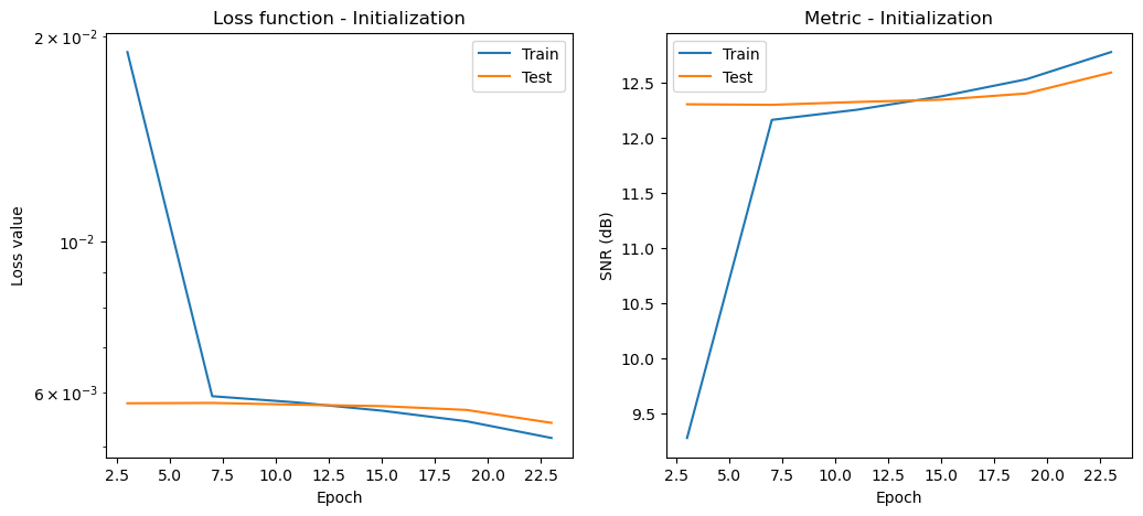
Check for iterated trained model. If not found, construct MoDLNet model, using only one iteration (depth) in model and few CG iterations for faster intialization. Run first stage (initialization) training loop followed by a second stage (depth iterations) training loop.
[8]:
channels = train_ds["image"].shape[-1]
workdir2 = os.path.join(
    os.path.expanduser("~"), ".cache", "scico", "examples", "modl_dcnv_out", "iterated"
)

stats_object_ini = None
stats_object = None

checkpoint_files = []
for dirpath, dirnames, filenames in os.walk(workdir2):
    checkpoint_files = [fn for fn in filenames]

if len(checkpoint_files) > 0:
    model = sflax.MoDLNet(
        operator=opBlur,
        depth=model_conf["depth"],
        channels=channels,
        num_filters=model_conf["num_filters"],
        block_depth=model_conf["block_depth"],
        cg_iter=model_conf["cg_iter"],
    )

    train_conf["workdir"] = workdir2
    train_conf["post_lst"] = [lmbdapos]
    # Construct training object
    trainer = sflax.BasicFlaxTrainer(
        train_conf,
        model,
        train_ds,
        test_ds,
    )
    start_time = time()
    modvar, stats_object = trainer.train()
    time_train = time() - start_time
    time_init = 0.0
    epochs_init = 0
else:
    # One iteration (depth) in model and few CG iterations
    model = sflax.MoDLNet(
        operator=opBlur,
        depth=1,
        channels=channels,
        num_filters=model_conf["num_filters"],
        block_depth=model_conf["block_depth"],
        cg_iter=model_conf["cg_iter"],
    )
    # First stage: initialization training loop.
    workdir1 = os.path.join(os.path.expanduser("~"), ".cache", "scico", "examples", "modl_dcnv_out")
    train_conf["workdir"] = workdir1
    train_conf["post_lst"] = [lmbdapos]
    # Construct training object
    trainer = sflax.BasicFlaxTrainer(
        train_conf,
        model,
        train_ds,
        test_ds,
    )

    start_time = time()
    modvar, stats_object_ini = trainer.train()
    time_init = time() - start_time
    epochs_init = train_conf["num_epochs"]

    print(
        f"{'MoDLNet init':18s}{'epochs:':2s}{train_conf['num_epochs']:>5d}{'':3s}"
        f"{'time[s]:':21s}{time_init:>7.2f}"
    )

    # Second stage: depth iterations training loop.
    model.depth = model_conf["depth"]
    train_conf["workdir"] = workdir2
    # Construct training object, include current model parameters
    trainer = sflax.BasicFlaxTrainer(
        train_conf,
        model,
        train_ds,
        test_ds,
        variables0=modvar,
    )

    start_time = time()
    modvar, stats_object = trainer.train()
    time_train = time() - start_time
channels: 1 training signals: 416 testing signals: 64 signal size: 256
Network Structure:
+------------------------------------------+----------------+--------+-----------+--------+
| Name | Shape | Size | Mean | Std |
+------------------------------------------+----------------+--------+-----------+--------+
| ResNet_0/BatchNorm_0/bias | (1,) | 1 | 0.0 | 0.0 |
| ResNet_0/BatchNorm_0/scale | (1,) | 1 | 1.0 | 0.0 |
| ResNet_0/ConvBNBlock_0/BatchNorm_0/bias | (64,) | 64 | 0.0 | 0.0 |
| ResNet_0/ConvBNBlock_0/BatchNorm_0/scale | (64,) | 64 | 1.0 | 0.0 |
| ResNet_0/ConvBNBlock_0/Conv_0/kernel | (3, 3, 1, 64) | 576 | -0.00161 | 0.0603 |
| ResNet_0/ConvBNBlock_1/BatchNorm_0/bias | (64,) | 64 | 0.0 | 0.0 |
| ResNet_0/ConvBNBlock_1/BatchNorm_0/scale | (64,) | 64 | 1.0 | 0.0 |
| ResNet_0/ConvBNBlock_1/Conv_0/kernel | (3, 3, 64, 64) | 36,864 | 0.000163 | 0.0418 |
| ResNet_0/ConvBNBlock_2/BatchNorm_0/bias | (64,) | 64 | 0.0 | 0.0 |
| ResNet_0/ConvBNBlock_2/BatchNorm_0/scale | (64,) | 64 | 1.0 | 0.0 |
| ResNet_0/ConvBNBlock_2/Conv_0/kernel | (3, 3, 64, 64) | 36,864 | -1.38e-05 | 0.0417 |
| ResNet_0/Conv_0/kernel | (3, 3, 64, 1) | 576 | -0.0018 | 0.0585 |
| lmbda | (1,) | 1 | 0.5 | 0.0 |
+------------------------------------------+----------------+--------+-----------+--------+
Total weights: 75,267
Batch Normalization:
+-----------------------------------------+-------+------+------+-----+
| Name | Shape | Size | Mean | Std |
+-----------------------------------------+-------+------+------+-----+
| ResNet_0/BatchNorm_0/mean | (1,) | 1 | 0.0 | 0.0 |
| ResNet_0/BatchNorm_0/var | (1,) | 1 | 1.0 | 0.0 |
| ResNet_0/ConvBNBlock_0/BatchNorm_0/mean | (64,) | 64 | 0.0 | 0.0 |
| ResNet_0/ConvBNBlock_0/BatchNorm_0/var | (64,) | 64 | 1.0 | 0.0 |
| ResNet_0/ConvBNBlock_1/BatchNorm_0/mean | (64,) | 64 | 0.0 | 0.0 |
| ResNet_0/ConvBNBlock_1/BatchNorm_0/var | (64,) | 64 | 1.0 | 0.0 |
| ResNet_0/ConvBNBlock_2/BatchNorm_0/mean | (64,) | 64 | 0.0 | 0.0 |
| ResNet_0/ConvBNBlock_2/BatchNorm_0/var | (64,) | 64 | 1.0 | 0.0 |
+-----------------------------------------+-------+------+------+-----+
Total weights: 386
Initial compilation, which might take some time ...
Initial compilation completed.
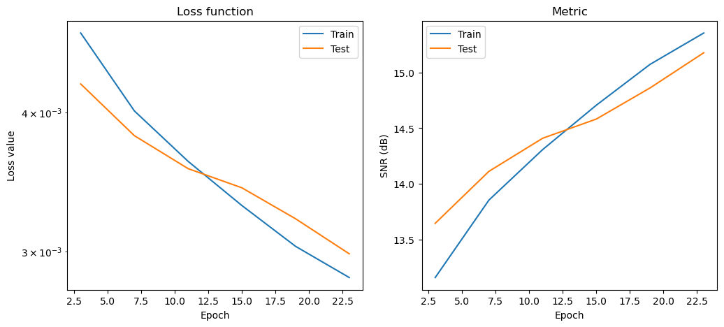
Epoch Time Train_LR Train_Loss Train_SNR Eval_Loss Eval_SNR
---------------------------------------------------------------------
3 9.02e+00 0.010000 0.018963 9.28 0.005786 12.30
7 1.24e+01 0.010000 0.005926 12.16 0.005793 12.30
11 1.45e+01 0.010000 0.005802 12.25 0.005758 12.32
15 1.63e+01 0.010000 0.005643 12.37 0.005731 12.34
19 1.83e+01 0.010000 0.005445 12.53 0.005657 12.40
23 2.03e+01 0.010000 0.005146 12.77 0.005416 12.59
MoDLNet init epochs: 25 time[s]: 22.29
channels: 1 training signals: 416 testing signals: 64 signal size: 256
Network Structure:
+------------------------------------------+----------------+--------+-----------+----------+
| Name | Shape | Size | Mean | Std |
+------------------------------------------+----------------+--------+-----------+----------+
| ResNet_0/BatchNorm_0/bias | (1,) | 1 | -0.0253 | 0.0 |
| ResNet_0/BatchNorm_0/scale | (1,) | 1 | 0.683 | 0.0 |
| ResNet_0/ConvBNBlock_0/BatchNorm_0/bias | (64,) | 64 | -2.41e-05 | 0.00088 |
| ResNet_0/ConvBNBlock_0/BatchNorm_0/scale | (64,) | 64 | 1.0 | 0.00101 |
| ResNet_0/ConvBNBlock_0/Conv_0/kernel | (3, 3, 1, 64) | 576 | 1.16e-05 | 0.0607 |
| ResNet_0/ConvBNBlock_1/BatchNorm_0/bias | (64,) | 64 | 7.48e-05 | 0.000618 |
| ResNet_0/ConvBNBlock_1/BatchNorm_0/scale | (64,) | 64 | 1.0 | 0.000836 |
| ResNet_0/ConvBNBlock_1/Conv_0/kernel | (3, 3, 64, 64) | 36,864 | 0.000214 | 0.0418 |
| ResNet_0/ConvBNBlock_2/BatchNorm_0/bias | (64,) | 64 | 8.59e-05 | 0.000627 |
| ResNet_0/ConvBNBlock_2/BatchNorm_0/scale | (64,) | 64 | 1.0 | 0.000788 |
| ResNet_0/ConvBNBlock_2/Conv_0/kernel | (3, 3, 64, 64) | 36,864 | -1.63e-05 | 0.0417 |
| ResNet_0/Conv_0/kernel | (3, 3, 64, 1) | 576 | -0.0028 | 0.0587 |
| lmbda | (1,) | 1 | 0.0315 | 0.0 |
+------------------------------------------+----------------+--------+-----------+----------+
Total weights: 75,267
Batch Normalization:
+-----------------------------------------+-------+------+-----------+--------+
| Name | Shape | Size | Mean | Std |
+-----------------------------------------+-------+------+-----------+--------+
| ResNet_0/BatchNorm_0/mean | (1,) | 1 | -0.69 | 0.0 |
| ResNet_0/BatchNorm_0/var | (1,) | 1 | 3.44 | 0.0 |
| ResNet_0/ConvBNBlock_0/BatchNorm_0/mean | (64,) | 64 | -0.000142 | 0.0511 |
| ResNet_0/ConvBNBlock_0/BatchNorm_0/var | (64,) | 64 | 0.00502 | 0.0036 |
| ResNet_0/ConvBNBlock_1/BatchNorm_0/mean | (64,) | 64 | 0.0558 | 0.491 |
| ResNet_0/ConvBNBlock_1/BatchNorm_0/var | (64,) | 64 | 0.402 | 0.317 |
| ResNet_0/ConvBNBlock_2/BatchNorm_0/mean | (64,) | 64 | -0.00125 | 0.409 |
| ResNet_0/ConvBNBlock_2/BatchNorm_0/var | (64,) | 64 | 0.434 | 0.338 |
+-----------------------------------------+-------+------+-----------+--------+
Total weights: 386
Initial compilation, which might take some time ...
Initial compilation completed.
Epoch Time Train_LR Train_Loss Train_SNR Eval_Loss Eval_SNR
---------------------------------------------------------------------
3 9.58e+00 0.010000 0.004716 13.16 0.004243 13.65
7 1.51e+01 0.010000 0.004012 13.86 0.003812 14.11
11 1.81e+01 0.010000 0.003614 14.31 0.003560 14.41
15 2.11e+01 0.010000 0.003298 14.71 0.003422 14.58
19 2.41e+01 0.010000 0.003031 15.07 0.003209 14.86
23 2.73e+01 0.010000 0.002841 15.35 0.002984 15.18
Evaluate on testing data.
[9]:
del train_ds["image"]
del train_ds["label"]

fmap = sflax.FlaxMap(model, modvar)
del model, modvar

maxn = test_nimg // 4
start_time = time()
output = fmap(test_ds["image"][:maxn])
time_eval = time() - start_time
output = np.clip(output, a_min=0, a_max=1.0)
Evaluate trained model in terms of reconstruction time and data fidelity.
[10]:
total_epochs = epochs_init + train_conf["num_epochs"]
total_time_train = time_init + time_train
snr_eval = metric.snr(test_ds["label"][:maxn], output)
psnr_eval = metric.psnr(test_ds["label"][:maxn], output)
print(
    f"{'MoDLNet training':18s}{'epochs:':2s}{total_epochs:>5d}{'':21s}"
    f"{'time[s]:':10s}{total_time_train:>7.2f}"
)
print(
    f"{'MoDLNet testing':18s}{'SNR:':5s}{snr_eval:>5.2f}{' dB'}"
    f"{'':3s}{'PSNR:':6s}{psnr_eval:>5.2f}{' dB'}{'':3s}{'time[s]:':10s}{time_eval:>7.2f}"
)
MoDLNet training  epochs:   50                     time[s]:    51.20
MoDLNet testing   SNR: 16.13 dB   PSNR: 23.21 dB   time[s]:     4.78
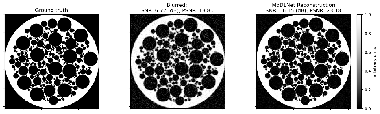
Plot comparison.
[11]:
np.random.seed(123)
indx = np.random.randint(0, high=maxn)

fig, ax = plot.subplots(nrows=1, ncols=3, figsize=(15, 5))
plot.imview(test_ds["label"][indx, ..., 0], title="Ground truth", cbar=None, fig=fig, ax=ax[0])
plot.imview(
    test_ds["image"][indx, ..., 0],
    title="Blurred: \nSNR: %.2f (dB), PSNR: %.2f"
    % (
        metric.snr(test_ds["label"][indx, ..., 0], test_ds["image"][indx, ..., 0]),
        metric.psnr(test_ds["label"][indx, ..., 0], test_ds["image"][indx, ..., 0]),
    ),
    cbar=None,
    fig=fig,
    ax=ax[1],
)
plot.imview(
    output[indx, ..., 0],
    title="MoDLNet Reconstruction\nSNR: %.2f (dB), PSNR: %.2f"
    % (
        metric.snr(test_ds["label"][indx, ..., 0], output[indx, ..., 0]),
        metric.psnr(test_ds["label"][indx, ..., 0], output[indx, ..., 0]),
    ),
    fig=fig,
    ax=ax[2],
)
divider = make_axes_locatable(ax[2])
cax = divider.append_axes("right", size="5%", pad=0.2)
fig.colorbar(ax[2].get_images()[0], cax=cax, label="arbitrary units")
fig.show()
Plot convergence statistics. Statistics are generated only if a training cycle was done (i.e. if not reading final epoch results from checkpoint).
[12]:
if stats_object is not None and len(stats_object.iterations) > 0:
    hist = stats_object.history(transpose=True)
    fig, ax = plot.subplots(nrows=1, ncols=2, figsize=(12, 5))
    plot.plot(
        np.vstack((hist.Train_Loss, hist.Eval_Loss)).T,
        x=hist.Epoch,
        ptyp="semilogy",
        title="Loss function",
        xlbl="Epoch",
        ylbl="Loss value",
        lgnd=("Train", "Test"),
        fig=fig,
        ax=ax[0],
    )
    plot.plot(
        np.vstack((hist.Train_SNR, hist.Eval_SNR)).T,
        x=hist.Epoch,
        title="Metric",
        xlbl="Epoch",
        ylbl="SNR (dB)",
        lgnd=("Train", "Test"),
        fig=fig,
        ax=ax[1],
    )
    fig.show()

# Stats for initialization loop
if stats_object_ini is not None and len(stats_object_ini.iterations) > 0:
    hist = stats_object_ini.history(transpose=True)
    fig, ax = plot.subplots(nrows=1, ncols=2, figsize=(12, 5))
    plot.plot(
        np.vstack((hist.Train_Loss, hist.Eval_Loss)).T,
        x=hist.Epoch,
        ptyp="semilogy",
        title="Loss function - Initialization",
        xlbl="Epoch",
        ylbl="Loss value",
        lgnd=("Train", "Test"),
        fig=fig,
        ax=ax[0],
    )
    plot.plot(
        np.vstack((hist.Train_SNR, hist.Eval_SNR)).T,
        x=hist.Epoch,
        title="Metric - Initialization",
        xlbl="Epoch",
        ylbl="SNR (dB)",
        lgnd=("Train", "Test"),
        fig=fig,
        ax=ax[1],
    )
    fig.show()